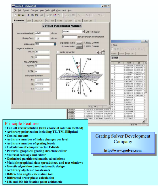
Gsolver 是一款強大的光柵結構設計軟體,軟體具有直觀的視覺化介面,可設計各種光柵結構剖面,如:方波全息光柵,閃耀光柵,正弦、梯形、三角形、三點折線式及其它許多結構光柵等。
它具有完全的三維向量代碼,模擬 計算精度高,材料齊全,另有全功能的展示版本下載試用,可滿足您的各種設計要求。GSolver 解答兩個半無限半空間介面(超基底和基底)上任意週期光柵結構內的 Maxwell 等式。
在使用者指定的截斷命令中作出唯一估算,確定光柵層介電常數(和非介電常數)的傅氏級數表示(Fourier series representation)中所使用的項數。GSolver 假設光柵結構由(任意空間解析度的)分段恒定結構確定,其中每個區域會被分配到一個均勻的等向性材料──一個恒定的折射率。
[GSolverLITE version includes only TE and TM polarization, and does not include crossed gratings
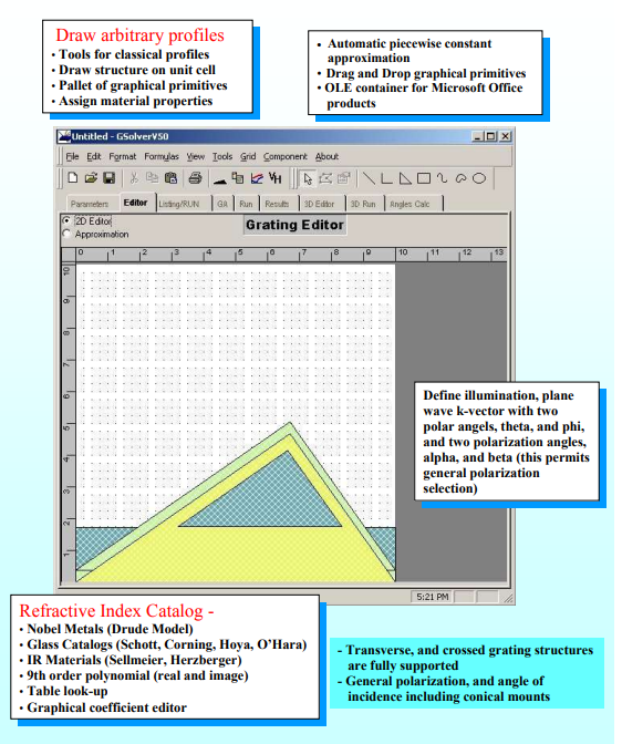
- A visual grating structure editor
- Automatic generation of common diffraction grating profiles including square wave holographic, blazed, sinusoidal, trapezoidal, triangular, 3-point polyline, and many others
- Arbitrary grating profile drawing tools, and general material pallet.
- Full 3-dimensional vector code
- Crossed grating analysis
- Analysis of arbitrary grating thickness, number of materials, and material index of refraction (defined by a real and imaginary part) including dielectrics and metals
- Automated generation of piecewise constant approximation
- Arbitrary grating complexity with multiple materials, coatings, buried structures, etc.
- Thin film analysis
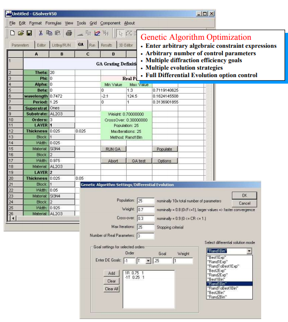
- Design optimizations with general genetic algorithm interface
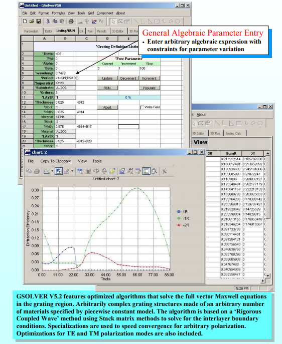
- Powerful algebraic language interface for generalized constraint definition
- Conical mounts and arbitrary polarization
- Legacy GS4 style grating editor
Binary Grating Example
This section gives a step-by-step example for creating a single binary layer grating (one layer with one index transition).
- Open GsolverV5.1
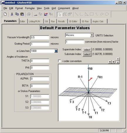
- The Parameters form is the global settings home. The substrate and superstrate materials may be selected here. (More details are found in the Dialogs chapter of the users manual.) Select a substrate and superstrate material by clicking on the appropriate select buttons.
- Enter the grating period (or lines/mm), wavelength, and other parameters. (A discussion of the angles is given in the Parameters Tab chapter.)
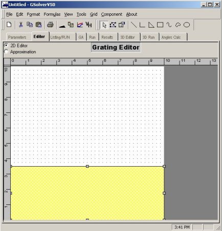
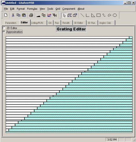
- Click on the Editor tab. Shown on this tab is the graphical working area called the canvas (see chapter 4). The substrate is located at 0 and below, referenced to the ruler on the left, and is not shown on the canvas.
- This example employs the square (rectangle) shape button to draw a rectangular structure. If not already present, use the menu item Tools->Customize to add the drawing tools to the toolbar. (See the section on toolbars if needed.)
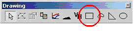
- Click on the square tool button. Place the mouse cursor anywhere on the active area of the canvas, and, while holding down the left mouse button, drag the mouse to create a rectangle on the canvas.
- Move the mouse cursor into the interior of the rectangle and right click. This brings up an item property menu. Select Properties.
- Select a material for the rectangular region just created. In principle, any shape may be made, and assigned a property. For overlapping shapes, the region on top is used when making the grating definition.
- Drag the rectangle to the bottom of the canvas so it rests on the substrate region.
- The units of the canvas are normalized to 1 grating period. The view region can be sized to any reasonable size, however the width of the canvas is 1 period no matter how the canvas is sized for display purposes. This is explained in detail in the Editor chapter.
- Recalling that periodic boundary conditions are assumed, the single rectangle drawn on the canvas represents a binary grating looking edge on. Once the grating is defined with the graphical editor, an internal piecewise-constant approximation can be created. This gives the representation used in the RCW analysis.
- Click on the Approximation radio button in the upper left corner of the canvas area to create the piecewise constant approximation. Each time this button is clicked, and only then, the internal representation of the piecewise constant construct is recalculated.
- The spatial resolution of the piecewise constant construct is determined by the canvas grid (see Editor Tab for greater detail). It can be made finer in two ways: 1) by changing the grid spacing by selecting Grid Properties from the Grid menu, which can also be activated by right clicking in the canvas area; or 2) by changing the canvas resolution (a number of view units equals one grating period), which can be accessed under the menu entry Edit->Canvas Properties. Also, the actual layer and inter-layer geometric dimensions of any piecewise constant feature are accessible, and modifiable on the Listing/RUN tab.
- Click the Run tab. This brings up the standard global parameter list similar to that of prior versions of GSolver. Using the check boxes, select one or several parameters, enter limits and then click the RUN button. The calculated results are shown on the Results Tab.
- Alternatively, click on the Listing/RUN tab to bring up the single parameter editable list option.
- On the Listing/RUN tab click the Populate button to load the list from the current internal piecewise constant construct. If the ‘Approximation’ button on the Editor form has not been clicked, this construct is empty, and so nothing will change. The piecewise constant listing is discussed in the Listing/RUN chapter.
- For this example the Listing/RUN will be used for a couple of simple calculations. To create a run with the angle of incidence changing. Enter the following formula into grid B2
=D5/2
All cell formulas begin with an equals sign (=) and are calculated immediately. [To toggle between formula view, and value view use the menu Formulas.>Formula View.] The formula engine included in GSolver is very extensive and powerful. It includes all common functions, and logicials, with logical conditional constructs. The formula engine is discussed in the Grid Formula chapter. Any cell can be used in any formula as long as nested iterations and a few restricted cells are avoided. - This Listing/RUN grid comes equipped with a single free parameter in cell D5. Enter the parameter increment and stop values as indicated in E5 and F5; set them to 0 and 80 respectively. This will cause the value of theta (formula entered in B2) to change from 0 to 40 degrees in steps of 0.5 degrees.
- Now click on the RUN button in cell D9. The first thing that happens is that GSolver cycles through the parameter range. For complicated formulas the increment and decrement buttons may be used to single step the grid computation to verify correct behavior.
- After the first run through, the parameter loop is reset, and then on each parameter increment the current grating list, as defined on the grid, is sent to the solver routines. The solution is written to the Results grid (Results tab).
- At the completion of the loop, the Results tab is displayed. Select any column(s) to graph by clicking on their headings. Multiple columns are selected using the shift and ctrl keys along with the mouse in the usual manner. The many options available for graphical display are discussed in the Graphing Options chapter.
- Return to the Listing/RUN tab. Reset the parameter D5 to 0 and change cell B2 to 10 for a fixed 10 degree incidence angle.
- Enter the following formula in cell B6 (wavelength):
=if(D5/100>.5,D5/100,.5)
This is a from of a conditional entry. The wavelength remains constant (0.5 microns) if D5/100<=0.5. Otherwise it changes linearly with D5 as given in the formula. - In cell B7 enter the following formula
=1.+D5/100.
This formula changes the grating period from 1 to 2 linearly as D5 changes from 0 to 100. - Change the orders field to 5.
- Click the Run button and examine the results.
Note that the thickness of any layer can be entered as a constant or through a formula on the grid listing. With this capability all film thicknesses (layers) can be accurately set; the finite grid resolution of the canvas does not limit layer thicknesses.
Blaze Grating Example:
For the Blaze grating use the tool button that shows a Blaze profile in black. This is a general tool that includes common grating design tasks.
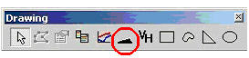
- From within the Editor tab, click on the Blaze tool button. This brings up the Custom Profile Construction dialog which includes Blaze, Triangle, Sinusoidal, Piecewise linear, and Piecewise spline.
- In the Blaze grid profile, select the desired blaze angle (change the default 35 in cell C3, or leave it as 35). Click OK.
- A blazed profile is created. A blaze grating profile is a right triangle. Select a material property for the triangle by right clicking it.
- At this point it is easy to create a conformal layer for this profile. Select the triangle shape just created with a mouse click, then hold down the control key, and click and drag the triangle. A copy of the triangle is created. Change the properties of the new triangle. Then send it behind the original triangle by right clicking the new triangle and using Order?Send to Back. Move the second triangle so that a thin conformal layer is created around the original triangle. The small gaps left in the lower right and left sides can be filled in with rectangles of the appropriate material settings.
- Click the Approximation button to create the piecewise constant approximation used by GSolver.
- Perform a grating calculation using the RUN or Listing/RUN tab.
Deep Grating Example:
GSolver is numerically stable for very deep gratings. To illustrate this create a simple binary grating in Aluminum. (See the User's Manual for guidance.)
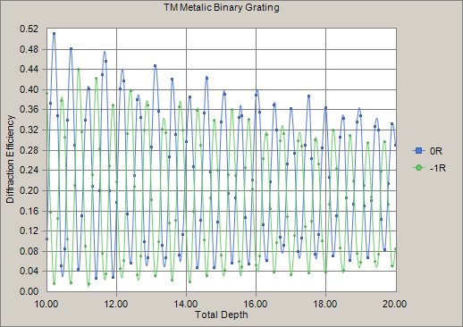
In this example I looked at the TE and TM polarization diffraction efficiency as a function grating (grove) depth. The aluminum substrate and 50% duty cycle aluminum grating had 800 lines/mm, 1 micron wavelength at 30 degrees incidence. 13 orders (total of 27) were retained.
The figure below shows the TE diffraction efficiency for a groove depth from 10 to 20 microns. This calculation could be extended to groove depths well beyond thousands of wavlengths without encountering numerical issues.
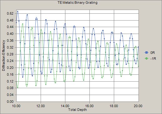
This next figure shows the same calculation for the TM mode.
Genetic Algorithm Thin File Design Example:
In this example the optimal AR (antireflection) coating thickness is sought for MgF2 on an Al2O3 substrate in air at normal incidence at 0.5 m wavelength.
See the User's Manual for screen shots and further details
- Open a new grating editor window
- Change the wavelength to 0.5 microns on the Parameter tab
- Change the Substrate material to Table: Al2O3
- Using the Rectangle tool in the Editor tab, create a thin film coating with width of the canvas and of arbitrary thickness.
- Set the rectangle material property to Table: MgF2
- Click the Approximation button which creates the piecewise grating data structure
- On the GA tab click Populate
- On the GA Options dialog, click the Options button, enter the following goal 0 R 0 1 (click Add)
- This indicates that the specular reflection has 0 energy the AR condition. Click OK
- In cell B12 enter the following formula =if(F5>0&&F5<0.2,F5,0)
- Change E5 to 0.4
- Click the GA test button to exercise the parameter selection and verify that the thickness is being updated, and constrained (non-negative and <0.2)
- Click RUN GA
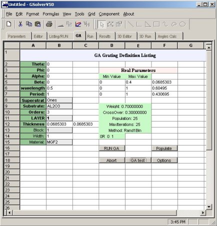
- The merit function (Best Energy) is updated each time a new minimum is found. The final result is updated to the listing. The result should be somewhere around 0.09
- Increasing the maximum constraint may cause the region of multiple minima to be reached. If so, multiple 'optimal' solutions may be found by executing the GA algorithm multiple times
While the GA is running, the current generation and best merit function are displayed. A merit function value of 0 indicates that an optimal solution has been found based on the goals given.
Upon completion the GA loads the values of the best parameters to the grid and creates a table of all the diffraction orders (-Orders to +Orders for T & R). This example is easily extendable to include multiple thin film layers. Simply add the materials in the Editor tab and use a separate parameter for each layer thickness.
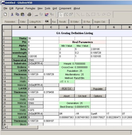
Genetic Algorithm Optimization of Sawtooth Profile Grating:
This example considers a sawtooth profile, such as might be cut by a DPT (diamond point turing) machine, in ZnSe. The problem is to find the optimal sawtooth profile (depth and period) to maximize transmission in the -1T order (-i order convention box on Parameters tab unchecked) for 3 micron wavelength, TE polarization, and for 30° incident light.
- Open a new grating editor window
- Change the wavelength to 3 and the substrate material to Herzberger: ZnSe(IRTR-4) and check the Lambda change update box. (This tells GSolver to update the index of refraction if the wavelength changes.)
- Change Theta to 30

- From the Editor tab, change the canvas properties (Edit Canvas Properties) so that Canvas height is 2. This allows for grating structures that are 2x the grating period, creating an approximation with a large number of layers for finer resolution.
- On the Editor tab, select the Custom Profile tool (black triangle)
- Select the General Sawtooth form, and change the angles to 35 and 90. Click OK.
- Select the newly created object and set its properties to Herzberger:ZnSe(IRTR-4). This should be the default if the substrate material was set.
- Select the shape and assure it is moved all the way to the bottom of the canvas. Then grab the top, center handle and stretch the shape so that it's height is 19 units (this equals 1.9*4 = 7.6 microns)
- Click the Approximation button
- Click the GA tab and Populate the grid
- Click the Options button and enter the goal as -1T 1 1 (-1T order, DE of 1, weight of 1). Click Add, then click OK.
- In cell B7 enter the following formula =if(f5>2&&f5<5,f5,4)
- This constrains the DE algorithm to only allow periods between 2 and 5 microns, and uses 4 microns as the default.
- Change D5 to 2 and E5 to 5
- Click the menu item Grid Thickness Formula, select All and enter the formula =if(f6>0&&f6<.2,f6,.1)
- This allows for a maximum thickness of 8 and a minimum of 0. Note there are 40 layers in the approximation.
- Set B10 (orders retained) to 8
- Set D6 to 0 and E6 to .2
- Click RUN GA
While the GA is running, the current generation is displayed together with the best merit function value. A value of 0 indicates that the goals were met perfectly.
For this example, a period of around 2.0, a total thickness of about 7.6, and an -1T order with approximately 96.9% efficiency are typical.
Change the mode settings under GA Options to examine the behavior of different DE evaluation schedules.
Following is a modification to the above example to find the best grating for simultaneously maximizing transmission, in the 1T and -1T, for thickness, period and angle of incidence. The best such configuration will have 1T = -1T = 0.5.
- Enter the following in B2 =if(F7>0&&F7<80,F7,40)
- Enter 0 in D7 and 80 in E7
- Change the goals on the Options dialog to 1T 0.5 1 and -1T 0.5 1
- Click RUN GA
A typical run may result in Theta = 2., Period = 2.7 and thickness = 2.7 with 1T = 42.% and -1T = 47%.